F Statistics
F3 Statistics
F3 statistics are a useful analytical tool to understand population relationships. F3 statistics, just as F4 and F2 statistics measure allele frequency correlations between populations and were introduced by Nick Patterson in his Patterson 2012
F3 statistics are used for two purposes: i) as a test whether a target population (C) is admixed between two source populations (A and B), and ii) to measure shared drift between two test populations (A and B) from an outgroup (C).
F3 statistics are in both cases defined as the product of allele frequency differences between population C to A and B, respectively:
Here, \(\langle\cdot\rangle\) denotes the average over all genotyped sites, and \(a, b\) and \(c\) denote the allele frequency for a given site in the three populations \(A, B\) and \(C\).
Admixture F3 Statistics
It can be shown that if that statistics is negative, it provides unambiguous proof that population C is admixed between populations A and B, as in the following phylogeny (taken from Figure 1 from Patterson 2012):
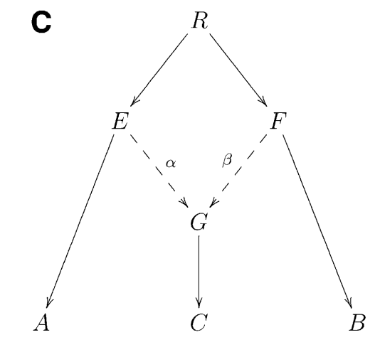
Intuitively, an F3 statistics becomes negative if the allele frequency of the target population (C) is on average intermediate between the allele frequencies of A and B. Consider as an extreme example a genomic site where \(a=0, b=1\) and \(c=0.5\). Then we have \((c-a)(c-b)=-0.25\), which is negative. So if the entire statistics is negative, it suggests that in many positions, the allele frequency \(c\) is indeed intermediate, suggesting admixture between the two sources.
Note
If an F3 statistics is not negative, it does not proof that there is no admixture!
We will use this statistics to test if Finnish are admixed between East and West, using different Eastern and Western sources. In the West, we use French, Icelandic, Lithuanian and Norwegian as source, and in the East we use Nganasan and one of the populations analysed in this workshop, Bolshoy Oleni Ostrov, a 3,500 year old group from the Northern Russian Kola-peninsula.
We use the software qp3Pop from AdmixTools, which similar to smartpca takes a parameter file:
genotypename:   input genotype file (in eigenstrat format)
snpname:        input snp file      (in eigenstrat format)
indivname:      input indiv file    (in eigenstrat format)
popfilename:    a file containing rows with three populations on each line A, B and C.
inbreed: YES
Here, the last option is necessary if we are analysing pseudo-diploid ancient data (which is the case here).
To prepare the popfilename, open a new file using Jupyter and enter:
Nganasan French Finnish
Nganasan Icelandic Finnish
Nganasan Lithuanian Finnish
Nganasan Norwegian Finnish
BolshoyOleniOstrov French Finnish
BolshoyOleniOstrov Icelandic Finnish
BolshoyOleniOstrov Lithuanian Finnish
BolshoyOleniOstrov Norwegian Finnish
Exercise
Prepare the parameter file with the input data as in the PCA session (see Principal Components Analysis (PCA)) and then run qp3Pop -p PARAMETER_FILE, where PARAMETERFILE should be replaced by your parameter file name. This will take about 3 minutes (see the ~/share/solutions/bash_commands notebook if you need a hint).
The results are in the output that you can view in the Notebook. The crucial bit should look like this:
                     Source 1             Source 2               Target           f_3       std. err           Z    SNPs
result:              Nganasan               French              Finnish     -0.004539       0.000510      -8.894  442567
result:              Nganasan            Icelandic              Finnish     -0.005297       0.000563      -9.404  427954
result:              Nganasan           Lithuanian              Finnish     -0.005062       0.000590      -8.574  426231
result:              Nganasan            Norwegian              Finnish     -0.004744       0.000569      -8.332  428161
result:    BolshoyOleniOstrov               French              Finnish     -0.002814       0.000444      -6.341  402958
result:    BolshoyOleniOstrov            Icelandic              Finnish     -0.002590       0.000486      -5.323  386418
result:    BolshoyOleniOstrov           Lithuanian              Finnish     -0.001523       0.000536      -2.840  384134
result:    BolshoyOleniOstrov            Norwegian              Finnish     -0.001553       0.000502      -3.092  386203
This output shows as first three columns the three populations A, B (sources) and C (target). Then the f3 statistics, which is negative in all cases tested here, a standard error, a Z score and the number of SNPs involved in the statistics.
The Z score is key: It gives the deviation of the f3 statistic from zero in units of the standard error. As general rule, a Z score of -3 or more suggests a significant rejection of the Null hypothesis that the statistic is not negative. In this case, all of the statistics are significantly negative, proving that Finnish have ancestral admixture of East and West Eurasian ancestry. Note that the statistics does not suggest when this admixture happened!
F4 Statistics
A different way to test for admixture is by “F4 statistics” (or “D statistics” which is very similar), also introduced in Patterson 2012.
F4 statistics are also defined in terms of correlations of allele frequency differences, similarly to F3 statistics (see above), but involving four different populations, not just three. Specifically we define
To understand the statistics, consider the following tree:
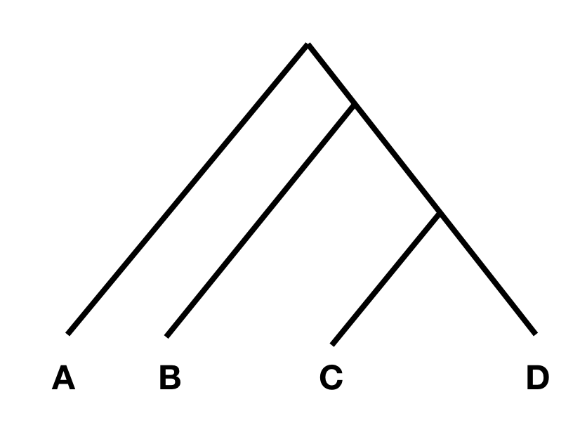
In this tree, without any additional admixture, the allele frequency difference between A and B should be completely independent from the allele frequency difference between C and D. In that case, F4(A, B; C, D) should be zero, or at least not statistically different from zero. However, if there was gene flow from C or D into A or B, the statistic should be different from zero. Specifically, if the statistic is significantly negative, it implies gene flow between either C and B, or D and A. If it is significantly positive, it implies gene flow between A and C, or B and D.
The way this statistic is often used, is to put a divergent outgroup as population A, for which we know for sure that there was no admixture into either C or D. With this setup, we can then test for gene flow between B and D (if the statistic is positive), or B and C (if it is negative).
Here, we can use this statistic to test for East Asian admixture in Finns, similarly to the test using Admixture F3 statistics above. We will use the qpDstat program from AdmixTools for that. We need to again prepare a population list file, this time with four populations (A, B, C, D). I suggest you open a new file and fill it with:
Mbuti Nganasan French Finnish
Mbuti Nganasan Icelandic Finnish
Mbuti Nganasan Lithuanian Finnish
Mbuti Nganasan Norwegian Finnish
Mbuti BolshoyOleniOstrov French Finnish
Mbuti BolshoyOleniOstrov Icelandic Finnish
Mbuti BolshoyOleniOstrov Lithuanian Finnish
Mbuti BolshoyOleniOstrov Norwegian Finnish
You can then use this file again in a parameter file, similar to the one prepared for qp3Pop above:
genotypename:   input genotype file (in eigenstrat format)
snpname:        input snp file      (in eigenstrat format)
indivname:      input indiv file    (in eigenstrat format)
popfilename:    a file containing rows with three populations on each line A, B and C.
f4mode: YES
Note that you cannot give the “inbreed” option here.
Exercise
Prepare the parameter file as suggested above and then run qpDstat -p PARAMETER_FILE, where PARAMETERFILE should be replaced by your parameter file name. This will take about 3 minutes (see the ~/share/solutions/bash_commands notebook if you need a hint).
The results should be (skipping some header lines):
result:      Mbuti   Nganasan     French    Finnish      0.002363     19.016   29254  27852 593124
result:      Mbuti   Nganasan  Icelandic    Finnish      0.001721     11.926   28915  27894 593124
result:      Mbuti   Nganasan Lithuanian    Finnish      0.001368      9.664   28745  27933 593124
result:      Mbuti   Nganasan  Norwegian    Finnish      0.001685     11.663   28933  27934 593124
result:      Mbuti BolshoyOleniOstrov     French    Finnish      0.001962     16.737   27249  26175 547486
result:      Mbuti BolshoyOleniOstrov  Icelandic    Finnish      0.001084      7.776   26876  26282 547486
result:      Mbuti BolshoyOleniOstrov Lithuanian    Finnish      0.000554      3.942   26683  26380 547486
result:      Mbuti BolshoyOleniOstrov  Norwegian    Finnish      0.000952      6.707   26873  26351 547486
Here, the key columns are columns 2, 3, 4 and 5, denoting A, B, C and D, and column 6 and 7, which denote the F4 statistic and the Z score, measuring significance in difference from zero.
As you can see, in all cases, the Z score is positive and larger than 3, indicating a significant deviation from zero, and implying gene flow between Nganasan and Finnish, and BolshoyOleniOstrov and Finnish, when compared to French, Icelandic, Lithuanian or Norwegian.
Outgroup F3 Statistics
Outgroup F3 statistics are a special case how to use F3 statistics. The definition is the same as for Admixture F3 statistics, but instead of a target C and two source populations A and B, one now gives an outgroup C and two test populations A and B.
To get an intuition for this statistics, consider the following tree:
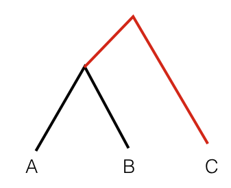
In this scenario, the statistic F3(A, B; C) measures the branch length from C to the common ancestor of A and B, coloured red. So this statistic is simply a measure of how closely two population A and B are related with each other, as measured from a distant outgroup. It is thus a similarity measure: The higher the statistic, the more genetically similar A and B are to one another.
We can use this statistic to measure for example the the genetic affinity to East Asia, by performing the statistic F3(Han, X; Mbuti), where Mbuti is a distant African population and acts as outgroup here, Han denote Han Chinese, and X denotes various European populations that we want to test.
You need to start, again, by preparing a list of population triples to be measured. I suggest the following list:
Han Chuvash Mbuti
Han Albanian Mbuti
Han Armenian Mbuti
Han Bulgarian Mbuti
Han Czech Mbuti
Han Druze Mbuti
Han English Mbuti
Han Estonian Mbuti
Han Finnish Mbuti
Han French Mbuti
Han Georgian Mbuti
Han Greek Mbuti
Han Hungarian Mbuti
Han Icelandic Mbuti
Han Italian_North Mbuti
Han Italian_South Mbuti
Han Lithuanian Mbuti
Han Maltese Mbuti
Han Mordovian Mbuti
Han Norwegian Mbuti
Han Orcadian Mbuti
Han Russian Mbuti
Han Sardinian Mbuti
Han Scottish Mbuti
Han Sicilian Mbuti
Han Spanish_North Mbuti
Han Spanish Mbuti
Han Ukrainian Mbuti
Han Levanluhta Mbuti
Han BolshoyOleniOstrov Mbuti
Han ChalmnyVarre Mbuti
Han Saami.DG Mbuti
which cycles through many populations from Europe, including the ancient individuals from Chalmny Varre, Bolshoy Oleni Ostrov and Levänluhta.
Exercise
Copy this list into a file, and prepare a parameter file for running qp3Pop, similar to the parameter file for admixture F3 statistics above, and run qp3Pop with that parameter file as above.
You should find this (skipping header lines from the output):
                      Source 1             Source 2               Target           f_3       std. err           Z    SNPs
result:                   Han              Chuvash                Mbuti      0.233652       0.002072     112.782  502678
result:                   Han             Albanian                Mbuti      0.215629       0.002029     106.291  501734
result:                   Han             Armenian                Mbuti      0.213724       0.001963     108.882  504370
result:                   Han            Bulgarian                Mbuti      0.216193       0.001979     109.266  504310
result:                   Han                Czech                Mbuti      0.218060       0.002002     108.939  504089
result:                   Han                Druze                Mbuti      0.209551       0.001919     109.205  510853
result:                   Han              English                Mbuti      0.216959       0.001973     109.954  504161
result:                   Han             Estonian                Mbuti      0.220730       0.002019     109.332  503503
result:                   Han              Finnish                Mbuti      0.223447       0.002044     109.345  502217
result:                   Han               French                Mbuti      0.216623       0.001969     110.012  509613
result:                   Han             Georgian                Mbuti      0.214295       0.001935     110.721  503598
result:                   Han                Greek                Mbuti      0.215203       0.001984     108.465  507475
result:                   Han            Hungarian                Mbuti      0.217894       0.001999     109.004  507409
result:                   Han            Icelandic                Mbuti      0.218683       0.002015     108.553  504655
result:                   Han        Italian_North                Mbuti      0.215332       0.001978     108.854  507589
result:                   Han        Italian_South                Mbuti      0.211787       0.002271      93.265  492400
result:                   Han           Lithuanian                Mbuti      0.219615       0.002032     108.098  503681
result:                   Han              Maltese                Mbuti      0.210359       0.001956     107.542  503985
result:                   Han            Mordovian                Mbuti      0.223469       0.002008     111.296  503441
result:                   Han            Norwegian                Mbuti      0.218873       0.002023     108.197  504621
result:                   Han             Orcadian                Mbuti      0.217773       0.002014     108.115  504993
result:                   Han              Russian                Mbuti      0.223993       0.001995     112.274  506525
result:                   Han            Sardinian                Mbuti      0.213230       0.001980     107.711  508413
result:                   Han             Scottish                Mbuti      0.218489       0.002039     107.145  499784
result:                   Han             Sicilian                Mbuti      0.212272       0.001975     107.486  505477
result:                   Han        Spanish_North                Mbuti      0.215885       0.002029     106.383  500853
result:                   Han              Spanish                Mbuti      0.213869       0.001975     108.297  513648
result:                   Han            Ukrainian                Mbuti      0.218716       0.002007     108.950  503981
result:                   Han           Levanluhta                Mbuti      0.236252       0.002383      99.123  263049
result:                   Han   BolshoyOleniOstrov                Mbuti      0.247814       0.002177     113.849  457102
result:                   Han         ChalmnyVarre                Mbuti      0.233499       0.002304     101.345  366220
result:                   Han             Saami.DG                Mbuti      0.236198       0.002274     103.852  489038
Now it’s time to plot these results using python.
Exercise
Copy the results (all lines from the output beginning with “results:”) into a text file, open a Jupyter python3 notebook and load the text file into a pandas dataframe, using pd.read_csv(FILENAME, delim_whitespace=True, names=["dummy", "A", "B", "C", "F3", "StdErr", "Z", "SNPS"]. View the resulting dataframe and make sure it looks correct.
A useful way to plot these results is by sorting them by the F3 statistics, and then plotting the test populations from left to right, beginning with the largest values. This code snippet should do the trick:
d=f3dat_han.sort_values(by="F3")
y = range(len(d))
plt.figure(figsize=(6, 8))
plt.errorbar(d["F3"], y, xerr=d["stderr"], fmt='o')
plt.yticks(y, d["B"]);
plt.xlabel("F3(Han, Test; Mbuti)");
Exercise
Use the above code snippet to plot the Outgroup F3 data. Google the errorbar and yticks functions from matplotlib if you want to know how they works.
You should get something like this:
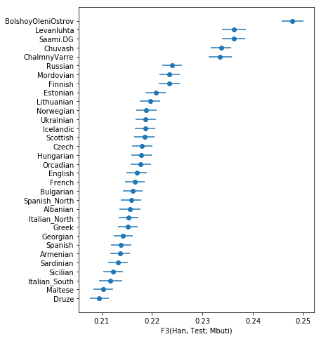
showing that, as expected, The ancient samples and modern Saami are most closely related to modern East Asians (as represented by Han) compared to many other Europeans.
Outgroup F3 Statistics Biplot
The above plot shows an intriguing cline of differential relatedness to Han in many Europeans. For example, would you have guessed that Icelandics are closer to Han than Armenians are to Han? This is very surprising, and it shows that European ancestry has a complex relationship to East Asians. To understand this better, you can read Patterson 2012, who makes some intriguing observations. Patterson and colleagues use Admixture F3 statistics and apply it to many populations world-wide. They summarise some population triples with the most negative F3 statistics in the following table:

There are many interesting results here, but one of the most striking one is the finding of F3(Sardinian, Karitiana; French), which is highly significantly negative. This statistics implies that French are admixed between Sardinians and Karitiana, a Native American population from Brazil. How is that possible? We can of course rule out any recent Native American backflow into Europe.
Patterson and colleagues explained this finding with hypothesising an ancient admixture event, from a Siberian population that contributed to both Europeans and to Native Americans. They termed that population the “Ancient North Eurasians (ANE)”. The following admixture graph was suggested:
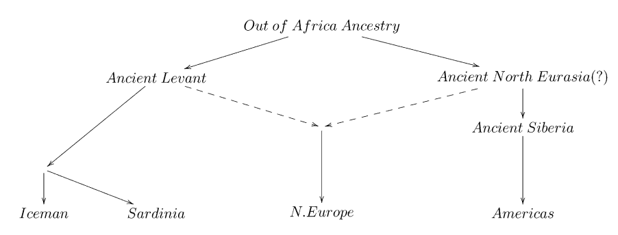
As you can see, the idea is that modern Central Europeans, such as French, are admixed between Southern Europeans (Sardinians) and ANE. The Ancient North Eurasians are a classic example for a “Ghost” population, a population which does not exist anymore in unmixed form, and from which we have no direct individual representative.
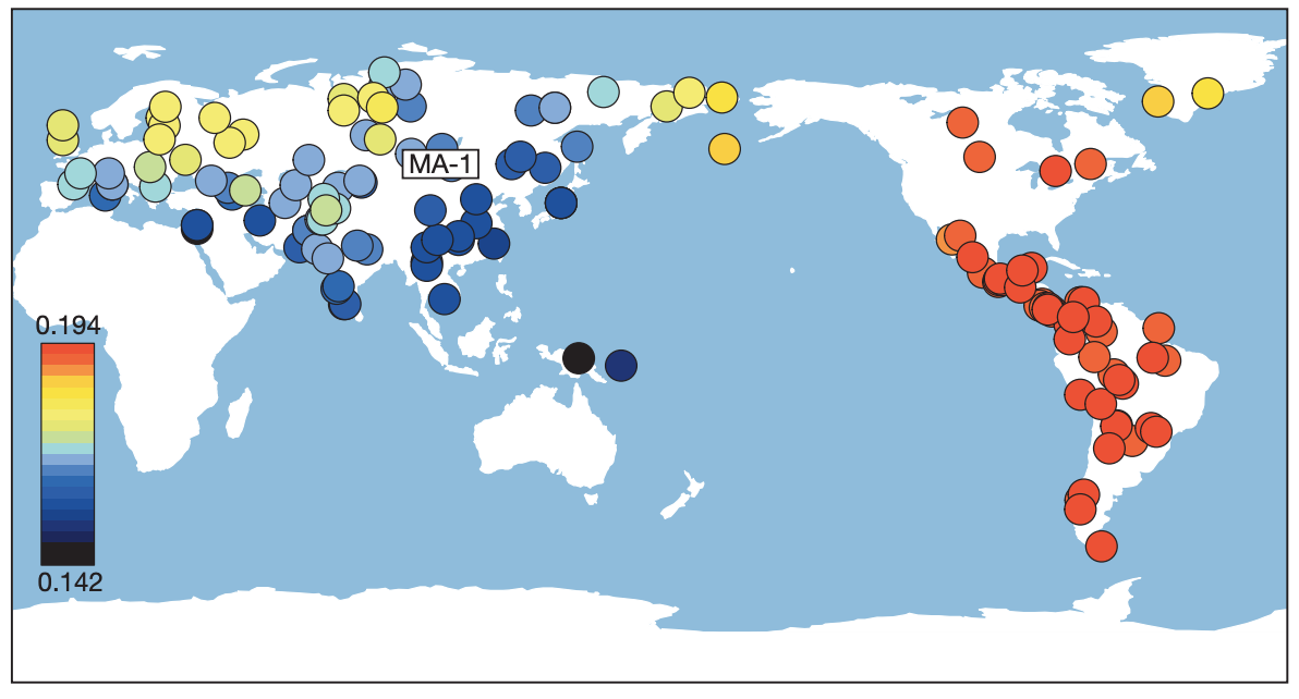
Amazingly, two years after the publication of Patterson 2012, the ANE ghost population was actually found: Raghavan et al. and colleagues, in 2014, published a paper called “Upper Palaeolithic Siberian genome reveals dual ancestry of Native Americans”. A 24,000 year old boy (called MA1) from the site of “Mal’ta” in Siberia was shown to have close genetic affinity with both Europeans and in particular Native Americans, just as proposed in Patterson 2012.
The affinities are summarised nicely in this figure from Raghavan et al.:
OK, so we now know that ancestry related to Native Americans contributed to European countries. Could that possibly explain the affinity of our ancient samples and Saami to Han Chinese in some way? To test this, we will run the same Outgroup F3 statistics as above, but this time not with Han but with MA1 as test population. Specifically, we run the following population triples in qp3Pop:
MA1_HG.SG Chuvash Mbuti
MA1_HG.SG Albanian Mbuti
MA1_HG.SG Armenian Mbuti
MA1_HG.SG Bulgarian Mbuti
MA1_HG.SG Czech Mbuti
MA1_HG.SG Druze Mbuti
MA1_HG.SG English Mbuti
MA1_HG.SG Estonian Mbuti
MA1_HG.SG Finnish Mbuti
MA1_HG.SG French Mbuti
MA1_HG.SG Georgian Mbuti
MA1_HG.SG Greek Mbuti
MA1_HG.SG Hungarian Mbuti
MA1_HG.SG Icelandic Mbuti
MA1_HG.SG Italian_North Mbuti
MA1_HG.SG Italian_South Mbuti
MA1_HG.SG Lithuanian Mbuti
MA1_HG.SG Maltese Mbuti
MA1_HG.SG Mordovian Mbuti
MA1_HG.SG Norwegian Mbuti
MA1_HG.SG Orcadian Mbuti
MA1_HG.SG Russian Mbuti
MA1_HG.SG Sardinian Mbuti
MA1_HG.SG Scottish Mbuti
MA1_HG.SG Sicilian Mbuti
MA1_HG.SG Spanish_North Mbuti
MA1_HG.SG Spanish Mbuti
MA1_HG.SG Ukrainian Mbuti
MA1_HG.SG Levanluhta Mbuti
MA1_HG.SG BolshoyOleniOstrov Mbuti
MA1_HG.SG ChalmnyVarre Mbuti
MA1_HG.SG Saami.DG Mbuti
where MA1_HG.SG is the cryptic name for the MA1 genome from Raghavan et al..
Exercise
Follow the same protocol as above: Copy the list into a file, prepare a parameter file for qp3Pop with that population triple list, and run qp3Pop. Copy the results (all lines beginning with “results:”) into a file and load it into python via pd.read_csv().
To test in what way the relationship to Han Chinese is correlated with the relationship with MA1, we will now plot the two statistics against each other in a scatter plot. We first have to merge the two outgroup-F3 datasets together. Here is the code including loading (assuming that the two F3 dataframes are called outgroupf3dat_Han and outgroupf3dat_MA1):
outgroupf3dat_Han = pd.read_csv("/home/training/work/outgroupF3_results_Han.txt",
                        delim_whitespace=True,
                        names=["dummy", "A", "B", "C", "F3", "stderr", "Z", "nSNPs"])
outgroupf3dat_MA1 = pd.read_csv("/home/training/work/outgroupF3_results_MA1.txt",
                        delim_whitespace=True,
                        names=["dummy", "A", "B", "C", "F3", "stderr", "Z", "nSNPs"])

outgroupf3dat_merged = outgroupf3dat_Han.merge(outgroupf3dat_MA1, on="B", suffixes=("_Han", "_MA1"))
Exercise
run the above merge command and check that it worked by viewing the resulting dataframe.
Finally, we can produce our bi-plot, using this code:
plt.figure(figsize=(10, 10))
plt.scatter(x=outgroupf3dat_merged["F3_Han"], y=outgroupf3dat_merged["F3_MA1"])
plt.xlabel("F3(Test, Han; Mbuti)");
plt.ylabel("F3(Test, MA1; Mbuti)");
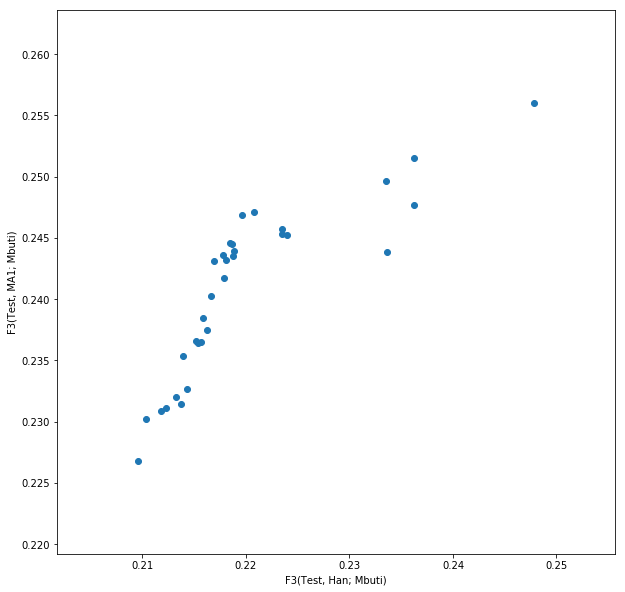
This should yield something like this:
This isn’t very useful, however, as we cannot see which point is which population. We can use the annotation function from matplotlib to add text labels to each point:
plt.figure(figsize=(10, 10))
plt.scatter(x=outgroupf3dat_merged["F3_Han"], y=outgroupf3dat_merged["F3_MA1"])
for i, row in outgroupf3dat_merged.iterrows():
    plt.annotate(row["B"], (row["F3_Han"], row["F3_MA1"]))
plt.xlabel("F3(Test, Han; Mbuti)");
plt.ylabel("F3(Test, MA1; Mbuti)");
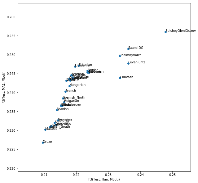
which should yield:
Exercise
Create this plot with the code snippets above.
The result shows that indeed the affinity to East Asians in the bulk of European contries can be explained by MA1-related ancestry. Most European countries have a linear relationship between their affinity to Han and their affinity to MA1. However, this is not true for our ancient samples from Fennoscandia and for modern Saami and Chuvash, who have extra affinity to Han not explained by MA1 (Lazaridis et al. 2014).