MSMC
Prerequisites
We first need to download some python scripts from the msmc-tools repository. To do that, go to your home directory and run git clone https://github.com/stschiff/msmc-tools
You should now have a directory called msmc-tools in your home-folder, as you can verify by running ls.
Data
All input data and intermediate files for this tutorial are at ~/share/MSMC-tutorial-files/.
For this lesson, we will use two trios from the 69 Genomes dataset by Complete Genomics. You will find the so called “MasterVarBeta” files for six individuals for chromosome 1 in the cg_data subdirectory in the tutorial files. Some information on the six samples: The first three form a father-mother-child trio from the West-African Yoruba, a people living in Nigeria. Here, NA19240 is the offspring, and NA19238 and NA19239 are the two parents. The second three samples form a father-mother-child trio from Utah (USA), with European ancestry. Here, NA12878 is the offspring, and NA12891 and NA12892 are the parents.
Generating consensus sequences for each sample
We will use the masterVar-files for each of the 6 samples, and use the cgCaller.py script in the msmc-tools repository to generate a VCF and a mask file for each individual from the masterVar file. For this, I suggest you write a little shell script that loops over all individuals:
#!/usr/bin/env bash

MASTERVARDIR=/path/to/sequence_data
OUTDIR=/path/to/output_files
CHR=chr1
for IND in NA19238 NA19239 NA19240 NA12878 NA12891 NA12892; do
    MASTERVAR=$(ls $MASTERVARDIR/masterVarBeta-$IND-*.tsv.chr1.bz2)
    OUT_MASK=$OUTDIR/$IND.$CHR.mask.bed.gz
    OUT_VCF=$OUTDIR/$IND.$CHR.vcf.gz
    ~/msmc-tools/cgCaller.py $CHR $IND $OUT_MASK $MASTERVAR | gzip -c > $OUT_VCF
done
Here, we restrict analysis only on chromosome 1 (which is called chr1 in the Complete Genomics data sets). Normally, you would also loop over chromosomes 1-22 in this script.
The line MASTERVAR=$(ls ...) uses bash command substitution to look for the masterVar file and store the result in the variable $MASTERVAR.
Copy the code above into a shell script, named for example runCGcaller.sh, adjust the paths, make it executable via chmod u+x runCGcaller.sh and run it. You should see log messages indicating the currently processed position in the chromosome. Chromosome 1 has about 250 million sites, so you can estimate the waiting time.
When finished (should take 10-20 minutes for all 6 samples), you should now have one *.mask.bed.gz and one *.vcf.gz file for each individual.
Combining samples
Some explanation on the generated files: The VCF file in each sample contains all sites at which at least one of the two chromosomes differs from the reference genome. Here is a sample:
##fileformat=VCFv4.1
##FORMAT=<ID=GT,Number=1,Type=String,Description="Phased Genotype">
#CHROM      POS     ID      REF     ALT     QUAL    FILTER  INFO    FORMAT  NA19238
chr1        38232   .       A       G       .       PASS    .       GT      1/1
chr1        41981   .       A       G       .       PASS    .       GT      1/1
chr1        47108   .       G       C       .       PASS    .       GT      1/0
chr1        47292   .       T       G       .       PASS    .       GT      1/0
chr1        49272   .       G       A       .       PASS    .       GT      1/1
chr1        51673   .       T       C       .       PASS    .       GT      1/0
chr1        52058   .       G       C       .       PASS    .       GT      1/0
This alone would not be enough information. MSMC is a Hidden Markov Model which uses the density of heterozygous sites (1/0 genotypes) to estimate the time to the most recent common ancestor. However, for a density you need not only a numerator but also a denominator, which in this case is the number of non-heterozygous sites, so typically homozygous reference alleles. Those are not part of this VCF file, for efficiency reasons. That’s why we have a Mask-file for each sample, that gives information in which regions in the genome could be called. Regions with not enough coverage or too low quality will be excluded. The first lines of such a mask look like this:
chr1        11093   11101
chr1        11137   11154
chr1        11203   11235
chr1        11276   11288
chr1        11319   11371
chr1        11378   11387
chr1        11437   11453
chr1        11481   11504
chr1        11511   11527
chr1        11568   11637
which gives a very detailed view on which regions could be called (2nd and 3rd column are begin and end).
There is one more mask that we need, which is the mappability mask. This mask defines regions in the reference genome in which we trust the mapping to be of high quality because the reference sequence is unique in that area. The mappability mask for chromosome 1 for the human reference GRCh37 is included in the Tutorial files. For all other chromosomes, this README includes a link to download them, but we won’t need them in this tutorial.
For generating the input files for MSMC, we will use a script called generate_multihetsep.py, which merges VCF and mask files together, and also performs simple trio-phasing. I will first show a command line that generates and MSMC input file for a single diploid sample NA12878:
#!/usr/bin/env bash

INDIR=/path/to/VCF/and/mask/files
OUTDIR=/path/to/output_files
MAPDIR=/path/to/mappability/mask
~/msmc-tools/generate_multihetsep.py --chr 1 --mask $INDIR/NA12878.mask.bed.gz \
    --mask $MAPDIR/hs37d5_chr1.mask.bed $INDIR/NA12878.vcf.gz > $OUTDIR/NA12878.chr1.multihetsep.txt
Here we have added the mask and VCF file of the NA12878 sample, and the mappability mask. I suggest you don’t actually run this because we won’t need this single-sample processing.
To process these two trios, we will use the two offspring samples only to phase the four parental chromosomes. You can do this with the trio option:
#!/usr/bin/env bash

INDIR=/path/to/VCF/and/mask/files
OUTDIR=/path/to/output_files
MAPDIR=/path/to/mappability/mask
generate_multihetsep.py --chr 1 \
    --mask $INDIR/NA12878.chr1.mask.bed.gz --mask $INDIR/NA12891.chr1.mask.bed.gz --mask $INDIR/NA12892.chr1.mask.bed.gz \
    --mask $INDIR/NA19240.chr1.mask.bed.gz --mask $INDIR/NA19238.chr1.mask.bed.gz --mask $INDIR/NA19239.chr1.mask.bed.gz \
    --mask $MAPDIR/hs37d5_chr1.mask.bed --trio 0,1,2 --trio 3,4,5 \
    $INDIR/NA12878.chr1.vcf.gz $INDIR/NA12891.chr1.vcf.gz $INDIR/NA12892.chr1.vcf.gz \
    $INDIR/NA19240.chr1.vcf.gz $INDIR/NA19238.chr1.vcf.gz $INDIR/NA19239.chr1.vcf.gz \
    > $OUTDIR/EUR_AFR.chr1.multihetsep.txt
Here we have first input all 6 calling masks, plus one mappability mask, then the two trio specifications (see ~/msmc-tools/generate_multihetsep.py -h for details), and then the 6 VCF files.
The first lines of the resulting “multihetsep” file should look like this:
1   68306   44      TTTCTCCT,TTTCCTTC
1   68316   10      CCCTTCCT,CCCTCTTC
1   87563   13      CCTTTTTT
1   570089  259     TTTTCCCC
1   752566  1058    AAAAAGAA
1   752721  83      GGGGGAGA
1   756781  596     GGGGGGGA
1   756912  113     AGAAAAAA
1   757103  26      CCCCCCCT
1   757734  84      TTTTTCTT
This is the input file for MSMC. The first two columns denote chromosome and position of a segregating site within the samples. The fourth column contains the 8 alleles in the 8 parental haplotypes of the four parents we put in. When there are multiple patterns separated by a comma, it means that phasing information is ambiguous, so there are multiple possible phasings. This can happen if all three members of a trio are heterozygous, which makes it impossible to separate the paternal and maternal allele.
The third column is special and I get a lot of questions about that column, so let me explain it as clearly as possible: The third column contains the number of called sites since the previous segregating site, including the current site. So for example, in the first row above, the first segregating site is at position 68306, but not all 68306 sites up to that site were called homozygous reference, but only 44. This is very important for MSMC, because it would otherwise assume that there was a huge homozygous segment spanning from 1 through 68306. Note that the very definition given above also means that the third column is always greater or equal to 1 (which is actually enforced by MSMC)!
Running MSMC2 for estimating the effective population size
MSMC’s purpose is to estimate coalescence rates between haplotypes through time. This can then be interpreted for example as the inverse effective population size through time. If the coalescence rate is estimated between subpopulations, another interpretation would be how separated the two populations became through time. In this tutorial, we will use both interpretations.
As a first step, we will use MSMC2 to estimate coalescence rates within the four African haplotypes alone, and within the four European haplotypes alone. Here is a short script running both these cases:
#!/usr/bin/env bash

INPUTDIR=/path/to/multihetsep/files
OUTDIR=/path/to/output/dir

msmc2 -p 1*2+15*1+1*2 -o $OUTDIR/EUR.msmc2 -I 0,1,2,3 $INPUTDIR/EUR_AFR.chr1.multihetsep.txt
msmc2 -p 1*2+15*1+1*2 -o $OUTDIR/AFR.msmc2 -I 4,5,6,7 $INPUTDIR/EUR_AFR.chr1.multihetsep.txt
Let’s go through the parameters one by one. The -p 1*2+15*1+1*2 option defines the time segment patterning. By default, MSMC uses 32 time segments, grouped as 1*2+25*1+1*2+1*3, which means that the first 2 segments are joined (forcing the coalescence rate to be the same in both segments), then 25 segments each with their own rate, and then again two groups of 2 and 3, respectively. MSMC2 run time and memory usage scales quadratically with the number of time segments. Here, since we are only analysing a single chromosome, you should reduce the number of segments to avoid overfitting. That’s why I set 18 segments, with two groups in the front and back. Grouping helps avoiding overfitting, as it reduces the number of free parameters.
The -o option denotes an output prefix. The three files generated by msmc will be called like this prefix with endings .final.txt, .loop.txt and .log.
The -I option denotes the 0-based indices of the haplotypes analysed. In our case we have 8 haplotypes, the first four being of European ancestry, the latter of African ancestry. In the first run we estimate coalescence rates within the European chromosomes (indices 0,1,2,3), and in the second case within the African chromosomes (indices 4,5,6,7). The last argument to msmc2 is the multihetsep file. Normally you would run it on all 22 chromosomes, and in that case you would simply give all those 22 files in a row.
On one processors, each of those runs will take about one hour, so that’s too long to actually run it, but you should at least test whether it starts alright and then kill the job using CTRL-C. The output files of the runs are available in the tutorial files.
Estimating population separation history
Above we have run MSMC on each population individually. In order to better understand when and how the two ancestral populations separated, we will use MSMC to estimate the coalescence rate across populations. Here is a script for this run:
#!/usr/bin/env bash

INPUTDIR=/path/to/multihetsep/files
OUTDIR=/path/to/output/dir

msmc2 -I 0-4,0-5,1-4,1-5 -s -p 1*2+15*1+1*2 -o $OUTDIR/AFR_EUR.msmc2 $INPUTDIR/EUR_AFR.chr1.multihetsep.txt
Here, I am running on all pairs between the first two parental chromosomes in each subpopulation, so -I 0-4,0-5,1-4,1-5. If you wanted to analyse all eight haplotypes (will take consiberably longer), you would have had to type -I 0-4,0-5,0-6,0-7,1-4,1-5,1-6,1-7,2-4,2-5,2-6,2-7,3-4,3-5,3-6,3-7.
The -s flag tells MSMC to skip sites with ambiguous phasing. As a rule of thumb: For population size estimates, we have found that unphased sites are not so much of a problem, but for cross-population analysis we typically remove those.
Plotting in Python
The result files from MSMC2 look like this:
time_index  left_time_boundary      right_time_boundary     lambda
0   0       2.61132e-06     2.93162
1   2.61132e-06     6.42208e-06     3043.06
2   6.42208e-06     1.19832e-05     3000.32
3   1.19832e-05     2.00987e-05     8353.98
4   2.00987e-05     3.19418e-05     12250.1
5   3.19418e-05     4.92247e-05     8982.41
...
Here, the first column denotes a simple index of all time segments, the second and third indicate the scaled start and end time for each time interval. The last column contains the scaled coalescence rate estimate in that interval.
Let’s first plot the effective population sizes with the following python code:
mu = 1.25e-8
gen = 30
afrDat = pd.read_csv("/path/to/AFR.msmc2.final.txt", delim_whitespace=True)
eurDat = pd.read_csv("/path/to/EUR.msmc2.final.txt", delim_whitespace=True)
plt.step(afrDat["left_time_boundary"]/mu*gen, (1/afrDat["lambda"])/(2*mu), label="AFR")
plt.step(eurDat["left_time_boundary"]/mu*gen, (1/eurDat["lambda"])/(2*mu), label="EUR")
plt.ylim(0,40000)
plt.xlabel("years ago");
plt.ylabel("effective population size");
plt.gca().set_xscale('log')
plt.legend()
Obviously, you have to adjust the path to the final result files under ~/share/MSMC-tutorial-files. The code produces this plot:
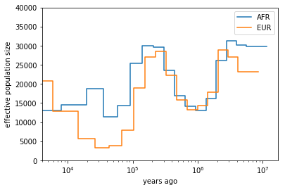
You can see that both ancestral population had similar effective population sizes before 200,000 years ago, after which the European ancestors experienced a severe population bottleneck. Of course, this is relatively low resolution because we are only analysing one chromosome, but the basic signal is already visible. Note that here we have scaled times and rates using a generation time of 30 years and a mutation rate of 1.25e-8, which are the same values as used in the initial publication on MSMC
For the cross-population results, we would like to plot the coalescence rate across populations relative to the values within the populations. However, since we have obtained these three rates independently, we have allowed MSMC2 to choose different time interval boundaries in each case, depending on the observed heterozygosity within and across populations. We therefore first have to use the script ~/msmc-tools/combinedCrossCoal.py:
#!/usr/bin/env bash

DIR=/path/to/msmc/results

combineCrossCoal.py $DIR/EUR_AFR.msmc2.final.txt $DIR/EUR.msmc2.final.txt \
    $DIR/AFR.msmc2.final.txt > $DIR/EUR_AFR.combined.msmc2.final.txt
The resulting file (also available under ~/share/MSMC-tutorial-files looks like this:
time_index  left_time_boundary      right_time_boundary     lambda_00       lambda_01       lambda_11
0   1.1893075e-06   4.75723e-06     1284.0425703    2.24322 2650.59574175
1   4.75723e-06     1.15451e-05     3247.01877925   2.24322 2940.90417746
2   1.15451e-05     2.12306e-05     7798.2270432    99.0725 2526.98957475
3   2.12306e-05     3.50503e-05     11261.3153077   2271.31 2860.21608183
4   3.50503e-05     5.47692e-05     8074.85679367   4313.17 3075.15793155
Here, instead of just one columns with coalescence rates, as before, we now have three. The first is the rate within population 0, the second across populations, the third within population 1.
OK, so we can now plot the relative cross-coalescence rate as a function of time:
mu = 1.25e-8
gen = 30
crossPopDat = pd.read_csv("/path/to/EUR_AFR.combined.msmc2.final.txt", delim_whitespace=True)
plt.step(crossPopDat["left_time_boundary"]/mu*gen, 2 * crossPopDat["lambda_01"] / (crossPopDat["lambda_00"] + crossPopDat["lambda_11"]))
plt.xlim(1000,500000)
plt.xlabel("years ago");
plt.ylabel("relative cross coalescence rate");
plt.gca().set_xscale('log')
which produces this plot:

where you can see that the separation of (West-African) and European ancestors began already 200,000 years ago. The two populations then became progressively more separated over time, reaching a mid-point of 0.5 around 80,000 years ago. Since about 45,000 years, the two population seem fully separated on this plot. Note that even in simulations with a sharp separation, MSMC would not produce an infinitely sharp separation curve, but introduces a “smear” around the true separation time, so this plot is compatible also with the assumption that the two populations where already fully separated around 60,000 years ago, even though the relative cross-coalescence rate is not zero at that point yet.